This is the second post in a series about geomagnetic storms as a global catastrophic risk. A paper covering the material in this series was just released.
My last post raised the specter of a geomagnetic storm so strong it would black out electric power across continent-scale regions for months or years, triggering an economic and humanitarian disaster.
How likely is that? One relevant source of knowledge is the historical record of geomagnetic disturbances, which is what this post considers. In approaching the geomagnetic storm issue, I had read some alarming statements to the effect that global society is overdue for the geomagnetic “Big One.” So I was surprised to find reassurance in the past. In my view, the most worrying extrapolations from the historical record do not properly represent it.
I hasten to emphasize that this historical analysis is only part of the overall geomagnetic storm risk assessment. Many uncertainties should leave us uneasy, from our incomplete understanding of the sun to the historically novel reliance of today’s grid operators on satellites that are themselves vulnerable to space weather. And since the scientific record stretches back only 30–150 years (depending on the indicator) and big storms happen about once a decade, the sample is too small to support sure extrapolations of extremes.
Nevertheless the historical record and claims based on it are the focus in this and the next post. I’ll examine four (kinds of) extrapolations that have been made from the record: from the last “Big One,” the Carrington event of 1859; from the July 2012 coronal mass ejection (CME) that might have caused a storm as large if it had hit Earth; a more complex extrapolation in Kappenman (2010); and the formal statistical extrapolation of Riley (2012). I’ll save the last for the next post.
The Carrington event
A series of CMEs starting in late August 1859 caused an extraordinary, global geomagnetic storm. It came to be named for astronomer Richard Carrington, who linked the events on earth to an intense solar flare he had observed on the sun hours before. The Carrington event produced spectacular auroras as far south, in the northern hemisphere, as San Salvador and as far north, in the southern hemisphere, as Santiago. Vivid reports came from around the world. Here is one from the Washington Territory of the US:
At 8 P.M. Aug. 28, 1859, a diffused light, without definite form, was observed a little east of north, covering about one-fourth of the heavens, which gradually increased to the west, sending across from east to west an arch of a whitish color, the arch itself being much brighter than the circumjacent light…At 9h25m P.M. strongly marked rays became visible, which rising from the horizon converged to a point on the arch a little south of the zenith, and in this position remained visible about one hour. The rays in the northwest were of a pink color, those in the southeast were purple, alternately brightening and fading to a whitish color. At midnight, all disappeared except the arch, and at intervals undulating flashes of light appeared not visible longer than three seconds. Occasionally streamers shot up from the horizon, the lower part disappearing before the upper part had reached the zenith. Sometimes these streamers were broad at the horizon, and came to a point near the zenith, and sometimes the reverse.
The storm hardly harmed human societies: it temporarily disrupted telegraph communications. Yet because of its apparent strength, the Carrington event of 1859 occupies a special place in the minds of those concerned about geomagnetic storms. It is the 1906 San Francisco earthquake, whose repetition is statistically inevitable. And next time global society may be much more vulnerable.
A critical question in assessing that vulnerability is: how much bigger was Carrington than the geomagnetic storms that have hit since the development of modern grids, which storms civilization has shrugged off? The paucity of high-quality scientific measurements from 1859 impedes comparisons (some magnetometers were operating, but went off scale). Scientists have made the most of the available data. The table below compares the Carrington event to more recent storms on several measures.
| Storm strength indicator | Carrington event, 1859 | Modern comparators | Sources |
|---|---|---|---|
| Lowest magnetic latitude where aurora visible | 23° | 29°, Mar. 1989 | Cliver and Svalgaard (2004), p. 417; Silverman (2006), p. 141 |
| Associated solar flare intensity (soft X-ray emissions) | 0.0045 W/m2 | 0.0035 W/m2, Nov. 2003 | Cliver and Dietrich (2013), pp. 2–3 |
| Transit time of CME to earth | 17.6 h | 14.6 h, Aug. 1972; 20.3 h, Oct. 2003 |
Cliver and Svalgaard (2004), Table III |
| Dst (low-latitude magnetic field depression) | –850 nT | –589 nT, Mar. 1989 | Siscoe, Crooker, and Clauer (2006); Kyoto University |
| W/m2 = watts/square meter; h = hours; nT = nanotesla | |||
Perhaps the most important comparison is in the last row. The storm-time disturbance (Dst) index represents the change in Earth’s magnetic field, as measured at four low-latitude observatories; it roughly proxies the overall geomagnetic impact of a storm. The Dst has only been compiled since 1957; scientists estimate that the Carrington event would have registered at roughly –850 nanotesla. As shown in the table, the biggest value on record is –589 nT; it occurred on March 14, 1989, which is when the Québec grid collapsed for some hours and permanently lost two transformers. (Last Tuesday a pretty-big CME drove the Dst to –195, the largest reading in 10 years.) This and the other comparisons in the table suggest that the Carrington storm was, conservatively, no more than twice as strong as modern events.
The July 2012 near-miss
Another important comparator is the major CME of July 23, 2012. That CME missed Earth because it left from what was then the far side of the sun. However, the NASA probe STEREO-A was travelling along earth’s orbit about 4 months ahead of the planet, and lay in the CME’s path, while STEREO-B, trailing four months behind earth, was also positioned to observe. The twin probes produced the best measurements ever of a Carrington-class solar event (Baker et al. 2013). Since the sun rotates about its axis in less than a month, had the CME come a couple of weeks sooner or later, it would have smashed into our planet.
Two numbers convey the power of the near-miss CME. First is its transit time to earth orbit: at just under 18 hours, almost exactly the same as in the Carrington event.[1] A slower CME on July 19 appears to have cleared the interplanetary medium of solar plasma, resulting in minimal slowdown of the big CME on July 23. The second number is the strength of the component of the CME’s magnetic field running parallel to earth’s. When a CME hits Earth, it strews the most magnetic chaos if its field parallels Earth’s (meaning that both point south); then it is like slamming together two magnetized toy trains the way they don’t want to go. The southward component of the magnetic field of the great July 2012 CME peaked at 50 nT. Here, however, “south” means perpendicular to Earth’s orbital plane. Since Earth’s spin axis is tilted 23.5° and its magnetic poles deviate from the spin poles by about another 10°, the southerly magnetic force of the near-miss CME, had it hit Earth, could have been more or less than 50 nT, depending on the exact time of day and year. Baker et al. (2013, p. 590) estimate the worst case as 70 nT south, relative to earth’s magnetic orientation.
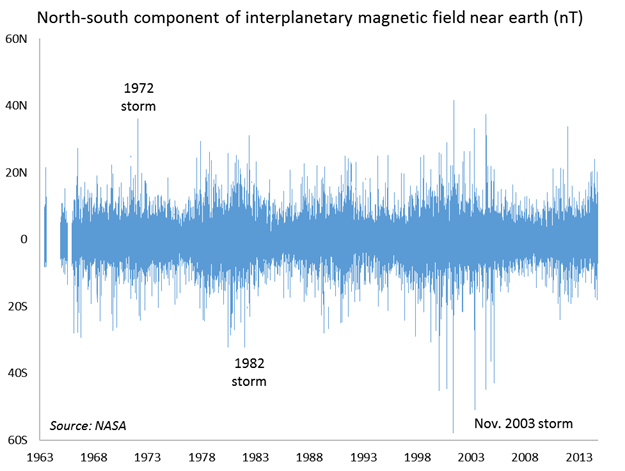
For comparison, the graph below shows the north-south component of the interplanetary magnetic field near earth since 1963, where north and south are also defined by the orientation of earth’s magnetic poles. Unfortunately, data are missing for the largest storm in the time range, the one of March 1989.[2] The graph does reveal a large northerly spike in 1972, which explains why that year’s great CME caused minimal disruption despite the record speed noted in the table above. Also shown are large southerly magnetic forces in storms of 1982 and 2003, the latter reaching 50 nT.
Given the near-miss CME’s speed, its magnetic field, and its density, how big a magnetic tempest would it have unleashed had it hit earth? Baker et al. (2013) estimate that it would have rated between –480 and –1182 on the Dst index, depending on the CME’s magnetic orientation relative to Earth’s at collision. Comparing the high value to the modern record of –589 again points to a benchmark worst-case storm as being twice as strong as anything experienced since the construction of modern grids.
In a companion paper, the same team of scientists ran computer simulations to develop a more sophisticated understanding of what would have happened if earth had been in STEREO-A’s place on July 23. Their results do not point clearly to a counterfactual catastrophe. “Had the 23 July CME hit Earth, there is a possibility that it could have produced comparable or slightly larger geomagnetically induced electric fields to those produced by previously observed Earth directed events such as the March 1989 storm or the Halloween 2003 storms.”
Kappenman’s factor of 10
In contrast, the prominent analyst John Kappenman has favored a factor of 10 to characterize the likely 100-year storm relative to the strongest recent storms.[3] Since this contrasts with my factor of two, I investigated the basis for the 10. It appears to arise as the ratio of two numbers.
One represents the worst disruption that geomagnetic storms have wrought in the modern age, meaning, again, the Québec blackout in March 1989. As Kappenman points out, just as the Richter scale doesn’t tell you everything about the destructive force of an earthquake in any given spot—local geology, distance from the epicenter, and building construction quality matter too—the Dst index doesn’t tell you everything about the capacity of a storm to induce electrical surges in any given place. What matters is not the total perturbation in the magnetic field, globally averaged, but the rate of magnetic field change from minute to minute along power lines of concern.[4] By the laws of electromagnetism, a changing magnetic field induces a voltage; and the faster the change, the bigger the voltage. In Québec in 1989, the rate of magnetic field change peaked at 479 nT/min (nanotesla per minute) according to Kappenman.
While I did not find a clear citation of source for this statistic, it looks highly plausible. The graph below, based on my extracts of magnetic observatory data, shows the maximum horizontal field changes at 58 stations on that day in 1989, based on measurements taken every minute, on the minute. Each 3-letter code represents an observatory; e.g., FRD is Fredericksburg, VA, and BFE is Brorfelde, Denmark.[5]
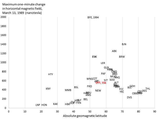
Ottawa (OTT, in red) recorded a peak change of 556 nT/min, between 9:50 and 9:51pm universal time, which is compatible with Kappenman’s 479 for nearby Québec. Brorfelde recorded the highest value, 1994 nT/min.
The other number in Kappenman’s factor-of-10 ratio represents the highest estimate we have of any per-minute magnetic field change before World War II, at least at a latitude low enough to concern Europe or North America. It comes from Karlstad, in southern Sweden, during the storm of May 13–15, 1921. The rate of change of the magnetic field was not measured there, but the electric field induced in a telegraph line was reportedly estimated at 20 volts/kilometer (V/km). Calibrating to modern observations, Kappenman calculates, “the 20 V/km observation…suggests the possibility that the disturbance intensity approached a level of 5000 nT/min.” Elsewhere Kappenman suggests 4800 nT/min. And 4800/479 is just about 10. That is, the worst case on record looks to be 10 times as bad as what caused the Québec blackout.
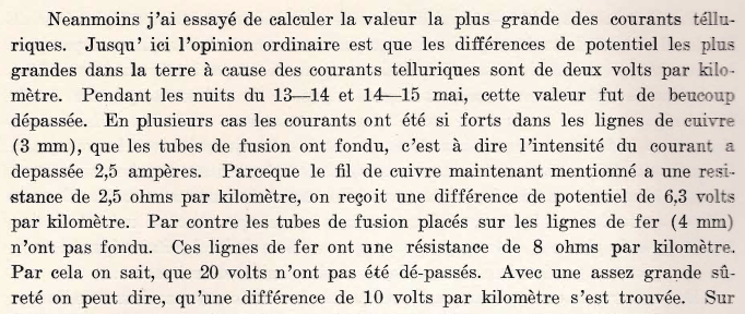
I have two doubts about this ratio. First, the top number appears to have been unintentionally increased by a scholarly game of telephone. As a source for the 20 V/km observation, Kappenman cites—and correctly represents—a 1992 conference paper by Elovaara et al., who write, “The earth surface potentials produced are typically characterized by the value 1 V/km, but in extreme cases much higher values has been recorded like 20 V/km in a wire communication system in Sweden in May 1922 [sic].” No source is given there; but Jarmo Elovaara pointed me to Sanders (1961) as likely. Indeed, there we read, “In May, 1921, during an outstanding magnetic storm, the largest earth-current voltages measured on wirelines in Sweden ranged from 6.3 to 20 v/km.” The cited source for that range is the “Earth Currents” article of the 1943 Encyclopedia Britannica, which states: “In May 1921, during an outstanding magnetic storm, Stenquist calculated from the fusing of some copper wires and the non-fusing of others that the largest earth current voltage in Sweden lay between 6.3 and 20 volts per kilometre.” “Stenquist” is David Stenquist, a Swedish telegraph engineer who in 1925 published Étude des Courants Telluriques (Study of Earth Currents). The pertinent passage thereof comes on page 54:
Translation:
Nevertheless I tried to calculate the largest value of telluric [earth] currents. Until now, standard opinion was that the largest potential differences in the earth because of telluric currents are two volts per kilometer. During the nights of May 13–14 and 14–15, this value was greatly exceeded. In many cases the currents were so strong in the lines of copper (3 mm [millimeters]), the conduits melted, i.e. the current exceeded 2.5 amps. Because the copper wire just mentioned had a resistance of 2.5 ohms per kilometer, we get a potential difference of 6.3 volts per kilometer. In contrast, the [fusion tubes?] placed on the iron lines (4 mm) did not melt. These iron lines have a resistance of 8 ohms per kilometer. So it is known that 20 volts did not occur. With a large enough security to speak, a difference of 10 volts per kilometer was found.
Stenquist believed the electric force field reached 10 V/km but explicitly rejected 20. Yet through the chain of citations, “20 volts n’ont pas été dé-passés” became “higher values has been recorded like 20 V/km.” Using Kappenman’s rule of thumb, Stenquist’s 10 V/km electrical force field suggests peaks of 2500 rather than 5000 nT/min of magnetic change on that dark and geomagnetically stormy night in Karlstad.
The second concern I have about the estimated ratio of 10 between magnetic fluctuations in the distant and recent past is that it appears to compare apples to oranges—an isolated, global peak value in one storm to a wide-area value in another. As we have already seen, the highest value observed in 1989 was not the 479 Kappenman uses to represent that storm but 1994 nT/min, in Brorfelde. And back in July 13–14, 1982, the Lovo observatory, at the same latitude as Karlstad, experienced 2688 nT/min, according to my calculations from the public data. Both instances were isolated: most observatories of comparable latitude reported much lower peaks. It is therefore not clear that the 1921 storm, with its isolated observation of 2500 nT/min, exceeded those of the 1980s at all, let alone by a factor of 10. Maximum magnetic changes and voltages may have been the same.
While there is apparently no evidence that fluctuations as great as 4800 nT/min have happened over large areas, Kappenman’s simulated 100-year storm scenario assumes that extremes of this order would occur across the US in a 5-degree band centered on 50° N geomagnetic latitude (an area 350 miles wide north-south, 3,000 long east-west)—4800 nT/min east of the Mississippi and 2400 nT/min to the west. The associated estimate that a 100-year storm would put 365 high-voltage transformers at risk of permanent damage, out of some 2,146 in service, affect regions home to 130 million people, and reduce economic output by trillions of dollars, entered an oft-cited National Research Council conference report. Yet to me, this seems like a highly unrepresentative extrapolation from history.
I found one other independent review of the Kappenman analysis. It was commissioned in 2011 by the US Department of Homeland Security from JASON, a group of scientists that advises the government on issues at the intersection of science and security. The JASON report concludes: “Because mitigation has not been widely applied to the U.S. electric grid, severe damage is a possibility, but a rigorous risk assessment has not been done. We are not convinced that the worst-case scenario of [Kappenman] is plausible. Nor is the analysis it is based on, using proprietary algorithms, suitable for deciding national policy….[W]e are unlikely to experience geomagnetic storms an order-of-magnitude more intense than those observed to date.”
Summary
Despite some spectacular reports from 1859 Carrington event and some equally spectacular scenario forecasts, to this point in our inquiry, the historical record appears surprisingly reassuring. There is little suggestion that the Carrington event—or any other in the last two centuries—was more than twice as strong as the biggest storms of recent decades, in 1982, 1989, and 2003. And civilization shrugged those off, with only a few high-voltage transformers taken out of commission. This does not prove geomagnetic storms pose no global catastrophic risk; like the JASON group, I don’t feel we can rule that out. But it does lead us to more focussed questions: What are the risks posed by a doubling of storm strength relative to recent experience? Under what circumstances would the effects be extremely disproportionate to the increase in magnetic disruption? What steps could be taken to prevent them?
In fact, I don’t feel that I have satisfactory answers to those questions. The area appears under-researched, and that may point to an opportunity for philanthropy.
But I get ahead of myself. In the next post, I will make a final approach on the historical record, this one more systematic and statistical. I think it’s important but it will not change the conclusion much.
Footnotes
[1] The eruption occurred at about 2:05 universal time on July 23, 2012. STEREO-A began to sense it around 21:00.
[2] Downloaded from cdaweb.sci.gsfc.nasa.gov/cdaweb/sp_phys, data set OMNI2_H0_MRG1HR, variable “1AU IP Bz (nT), GSM” (meaning 1 astronomical unit from sun, interplanetary magnetic field Z component, nanotesla, geocentric solar magnetospheric coordinates). Readings are hourly, with gaps.
[3] “Because the [1-in-100 year scenario] 4800nT/min threat environment is ~10 times larger than the peak March 1989 storm environment, this comparison also indicates that resulting GIC peaks will also in general be nearly 10 times larger as well” (Kappenman 2010, p. 4-12). “This disturbance level is nearly 10 times larger than the levels that precipitated the North American power system impacts of 13 March 1989” (Kappenman 2004). “Measured data has shown that storms with impulsive disturbance levels that are 4 to 10 times larger than those that impacted the North American grid in March 1989 have occurred before” (Kappenman 2012, p. 2).
[4] Pulkkinen et al. (2008) find that standard modeling approaches for translating geomagnetic disturbances into induced voltages are reasonably accurate using 1-minute time resolution data, with the modeled peak more than 80% of the true peak. Going to a cadence of 10 seconds eliminates the remaining gap.
[5] Plotted are all stations with data for the period in NOAA’s SPIDR system or the Nordic IMAGE network. Geomagnetic latitudes are from NASA’s geomagnetic coordinate calculator. A list and maps of observatories is here.