We’ve recently been writing about the shortcomings of formal cost-effectiveness estimation (i.e., trying to estimate how much good, as measured in lives saved, DALYs or other units, is accomplished per dollar spent). After conceptually arguing that cost-effectiveness estimates can’t be taken literally when they are not robust, we found major problems in one of the most prominent sources of cost-effectiveness estimates for aid, and generalized from these problems to discuss major hurdles to usefulness faced by the endeavor of formal cost-effectiveness estimation.
Despite these misgivings, we would be determined to make cost-effectiveness estimates work, if we thought this were the only way to figure out how to allocate resources for maximal impact. But we don’t. This post argues that when information quality is poor, the best way to maximize cost-effectiveness is to examine charities from as many different angles as possible – looking for ways in which their stories can be checked against reality – and support the charities that have a combination of reasonably high estimated cost-effectiveness and maximally robust evidence. This is the approach GiveWell has taken since our inception, and it is more similar to investigative journalism or early-stage research (other domains in which people look for surprising but valid claims in low-information environments) than to formal estimation of numerical quantities.
The rest of this post
- Conceptually illustrates (using the mathematical framework laid out previously) the value of examining charities from different angles when seeking to maximize cost-effectiveness.
- Discusses how this conceptual approach matches the approach GiveWell has taken since inception.
I don’t wish to present this illustration either as official GiveWell analysis or as “the reason” that we believe what we do. This is more of an illustration/explication of my views than a justification; GiveWell has implicitly (and intuitively) operated consistent with the conclusions of this analysis, long before we had a way of formalizing these conclusions or the model behind them. Furthermore, while the conclusions are broadly shared by GiveWell staff, the formal illustration of them should only be attributed to me.
The model
Suppose that:
- Your prior over the “good accomplished per $1000 given to a charity” is normally distributed with mean 0 and standard deviation 1 (denoted from this point on as N(0,1)). Note that I’m not saying that you believe the average donation has zero effectiveness; I’m just denoting whatever you believe about the impact of your donations in units of standard deviations, such that 0 represents the impact your $1000 has when given to an “average” charity and 1 represents the impact your $1000 has when given to “a charity one standard deviation better than average” (top 16% of charities).
- You are considering a particular charity, and your back-of-the-envelope initial estimate of the good accomplished by $1000 given to this charity is represented by X. It is a very rough estimate and could easily be completely wrong: specifically, it has a normally distributed “estimate error” with mean 0 (the estimate is as likely to be too optimistic as too pessimistic) and standard deviation X (so 16% of the time, the actual impact of your $1000 will be 0 or “average”).* Thus, your estimate is denoted as N(X,X).
The implications
I use “initial estimate” to refer to the formal cost-effectiveness estimate you create for a charity – along the lines of the DCP2 estimates or Back of the Envelope Guide estimates. I use “final estimate” to refer to the cost-effectiveness you should expect, after considering your initial estimate and making adjustments for the key other factors: your prior distribution and the “estimate error” variance around the initial estimate. The following chart illustrates the relationship between your initial estimate and final estimate based on the above assumptions.
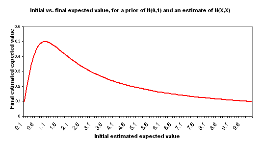
This is in some ways a counterintuitive result. A couple of ways of thinking about it:
- Informally: estimates that are “too high,” to the point where they go beyond what seems easily plausible, seem – by this very fact – more uncertain and more likely to have something wrong with them. Again, this point applies to very rough back-of-the-envelope style estimates, not to more precise and consistently obtained estimates.
- Formally: in this model, the higher your estimate of cost-effectiveness goes, the higher the error around that estimate is (both are represented by X), and thus the less information is contained in this estimate in a way that is likely to shift you away from your prior. This will be an unreasonable model for some situations, but I believe it is a reasonable model when discussing very rough (“back-of-the-envelope” style) estimates of good accomplished by disparate charities. The key component of this model is that of holding the “probability that the right cost-effectiveness estimate is actually ‘zero’ [average]” constant. Thus, an estimate of 1 has a 67% confidence interval of 0-2; an estimate of 1000 has a 67% confidence interval of 0-2000; the former is a more concentrated probability distribution.
Now suppose that you make another, independent estimate of the good accomplished by your $1000, for the same charity. Suppose that this estimate is equally rough and comes to the same conclusion: it again has a value of X and a standard deviation of X. So you have two separate, independent “initial estimates” of good accomplished, and both are N(X,X). Properly combining these two estimates into one yields an estimate with the same average (X) but less “estimate error” (standard deviation = X/sqrt(2)). Now the relationship between X and adjusted expected value changes:
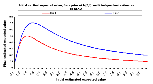
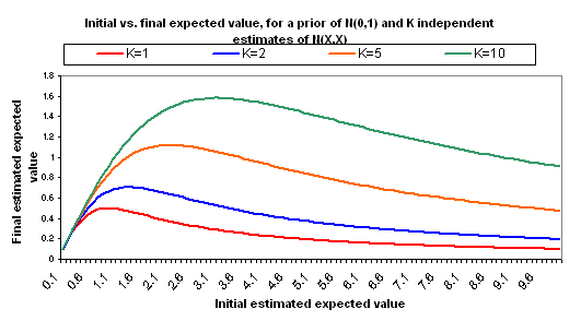
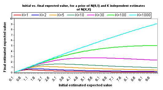
The following charts show what happens if you manage to collect even more independent cost-effectiveness estimates, each one as rough as the others, each one with the same midpoint as the others (i.e., each is N(X,X)).
A few other notes:
- The full calculations behind the above charts are available here (XLS). We also provide another Excel file that is identical except that it assumes a variance for each estimate of X/2, rather than X. This places “0” just inside your 95% confidence interval for the “correct” version of your estimate. While the inflection points are later and higher, the basic picture is the same.
- It is important to have a cost-effectiveness estimate. If the initial estimate is too low, then regardless of evidence quality, the charity isn’t a good one. In addition, very high initial estimates can imply higher potential gains to further investigation. However, “the higher the initial estimate of cost-effectiveness, the better” is not strictly true.
- Independence of estimates is key to the above analysis. In my view, different formal estimates of cost-effectiveness are likely to be very far from independent because they will tend to use the same background data and assumptions and will tend to make the same simplifications that are inherent to cost-effectiveness estimation (see previous discussion of these simplifications here and here).Instead, when I think about how to improve the robustness of evidence and thus reduce the variance of “estimate error,” I think about examining a charity from different angles – asking critical questions and looking for places where reality may or may not match the basic narrative being presented. As one collects more data points that support a charity’s basic narrative (and weren’t known to do so prior to investigation), the variance of the estimate falls, which is the same thing that happens when one collects more independent estimates. (Though it doesn’t fall as much with each new data point as it would with one of the idealized “fully independent cost-effectiveness estimates” discussed above.)
- The specific assumption of a normal distribution isn’t crucial to the above analysis. I believe (based mostly on a conversation with Dario Amodei) that for most commonly occurring distribution types, if you hold the “probability of 0 or less” constant, then as the midpoint of the “estimate/estimate error” distribution approaches infinity the distribution becomes approximately constant (and non-negligible) over the area where the prior probability is non-negligible, resulting in a negligible effect of the estimate on the prior.While other distributions may involve later/higher inflection points than normal distributions, the general point that there is a threshold past which higher initial estimates no longer translate to higher final estimates holds for many distributions.
number of people whose jobs produce the income necessary to give them and their families a relatively comfortable lifestyle (including health, nourishment, relatively clean and comfortable shelter, some leisure time, and some room in the budget for luxuries), but would have been unemployed or working completely non-sustaining jobs without the charity’s activities, per dollar per year. (Systematic differences in family size would complicate this.)
Early on, we weren’t sure of whether we would find good enough information to quantify these sorts of things. After some experience, we came to the view that most cost-effectiveness analysis in the world of charity is extraordinarily rough, and we then began using a threshold approach, preferring charities whose cost-effectiveness is above a certain level but not distinguishing past that level. This approach is conceptually in line with the above analysis.
It has been remarked that “GiveWell takes a deliberately critical stance when evaluating any intervention type or charity.” This is true, and in line with how the above analysis implies one should maximize cost-effectiveness. We generally investigate charities whose estimated cost-effectiveness is quite high in the scheme of things, and so for these charities the most important input into their actual cost-effectiveness is the robustness of their case and the number of factors in their favor. We critically examine these charities’ claims and look for places in which they may turn out not to match reality; when we investigate these and find confirmation rather than refutation of charities’ claims, we are finding new data points that support what they’re saying. We’re thus doing something conceptually similar to “increasing K” according to the model above. We’ve recently written about all the different angles we examine when strongly recommending a charity.
We hope that the content we’ve published over the years, including recent content on cost-effectiveness (see the first paragraph of this post), has made it clear why we think we are in fact in a low-information environment, and why, therefore, the best approach is the one we’ve taken, which is more similar to investigative journalism or early-stage research (other domains in which people look for surprising but valid claims in low-information environments) than to formal estimation of numerical quantities.
As long as the impacts of charities remain relatively poorly understood, we feel that focusing on robustness of evidence holds more promise than focusing on quantification of impact.
*This implies that the variance of your estimate error depends on the estimate itself. I think this is a reasonable thing to suppose in the scenario under discussion. Estimating cost-effectiveness for different charities is likely to involve using quite disparate frameworks, and the value of your estimate does contain information about the possible size of the estimate error. In our model, what stays constant across back-of-the-envelope estimates is the probability that the “right estimate” would be 0; this seems reasonable to me.
Comments
I think it’s worth pointing out some of the strange implications of a normal prior for charity cost-effectiveness.
For instance, it appears that one can save lives hundreds of times more cheaply through vaccinations in the developing world than through typical charity expenditures aimed at saving lives in rich countries, according to experiments, government statistics, etc.
But a normal distribution (assigns) a probability of one in tens of thousands that a sample will be more than 4 standard deviations above the median, and one in hundreds of billions that a charity will be more than 7 standard deviations from the median. The odds get tremendously worse as one goes on. If your prior was that charity cost-effectiveness levels were normally distributed, then no conceivable evidence could convince you that a charity could be 100x as good as the 90th percentile charity. The probability of systematic error or hoax would always be ludicrously larger than the chance of such an effective charity. One could not believe, even in hindsight, that paying for Norman Borlaug’s team to work on the Green Revolution, or administering smallpox vaccines (with all the knowledge of hindsight) actually did much more good than typical. The gains from resources like GiveWell would be small compared to acting like an index fund and distributing charitable dollars widely.
Such denial seems unreasonable to me, and I think to Holden. However, if one does believe that there have in fact been multiple interventions that turned out 100x as effective as the 90th percentile charity, then one should reject a normal prior. When a model predicts that the chance of something happening is less than 10^-100, and that thing goes on to happen repeatedly in the 20th century, the model is broken, and one should try to understand how it could be so wrong.
Another problem with the normal prior (and, to a lesser but still problematic extent, a log-normal prior) is that it would imply overconfident conclusions about the physical world.
For instance, consider threats of human extinction. Using measures like “lives saved” or “happy life-years produced,” counting future generations the gain of averting a human extinction scales with the expected future population of humanity. There are pretty well understood extinction risks with well understood interventions, where substantial progress has been made: with a trickle of a few million dollars per year (for a couple decades) in funding 90% of dinosaur-killer size asteroids were tracked and checked for future impacts on Earth. So, if future populations are large then using measures like happy life-years there will be at least some ultra-effective interventions.
If humanity can set up a sustainable civilization and harness a good chunk of the energy of the Sun, or colonize other stars, then really enormous prosperous populations could be created: see Nick Bostrom’s (paper) on astronomical waste for figures.
From this we can get something of a reductio ad absurdum for the normal prior on charity effectiveness. If we believed a normal prior then we could reason as follows:
1. If humanity has a reasonable chance of surviving to build a lasting advanced civilization, then some charity interventions are immensely cost-effective, e.g. the historically successful efforts in asteroid tracking.
2. By the normal (or log-normal) prior on charity cost-effectiveness, no charity can be immensely cost-effective (with overwhelming probability).
Therefore,
3. Humanity is doomed to premature extinction, stagnation, or an otherwise cramped future.
I find this “Charity Doomsday Argument” pretty implausible. Why should intuitions about charity effectiveness let us predict near-certain doom for humanity from our armchairs? Long-term survival of civilization on Earth and/or space colonization are plausible scenarios, not to be ruled out in this a priori fashion.
To really flesh out the strangely strong conclusion of these priors, suppose that we lived to see spacecraft intensively colonize the galaxy. There would be a detailed history leading up to this outcome, technical blueprints and experiments supporting the existence of the relevant technologies, radio communication and travelers from other star systems, etc. This would be a lot of evidence by normal standards, but the normal (or log-normal) priors would never let us believe our own eyes: someone who really held a prior like that would conclude they had gone insane or that some conspiracy was faking the evidence.
Yet if I lived through an era of space colonization, I think I could be convinced that it was real. I think Holden could be convinced that it was real. So a prior which says that space colonization is essentially impossible does not accurately characterize our beliefs.
Carl, I agree that it isn’t reasonable to literally have a normally distributed prior over the impact of charitable gifts as measured in something like “lives saved” or “DALYs saved.” However, a lognormally distributed prior over these things seems quite defensible, and all of the above analysis can be applied if you use something like “log of lives saved” as your unit for measuring impact.
As mentioned, the analysis should actually apply in broad outline even when another distribution (e.g., power-law) is used.
I used normal distributions to illustrate the concepts discussed here as simply as possible, without getting into the units in which one ought to denote impact. My aim was to illustrate the relative importance of quantified estimated impact and robustness of evidence (and the theoretical justification behind a “threshold” approach to cost-effectiveness estimates), not to provide specific numbers for people to use.
Note that we removed John Lawless’s comments, at his request, and will be following up with him by email.
Carl:
Good points. The rough, informal prior that I use is some kind of combination of normal, log-normal, and even more skewed distributions (eg power law). In particular, it can’t be normal as the right hand tail is clearly too thin. It can’t be log-normal as the left hand tail should give probability to negative effectivenesses and the right hand tail is still too thin (smallpox and the green revolution are good examples).
Holden: Interesting post. I have two comments:
(1) In the post you assume N(X,X) as the underlying distribution for an estimate of X. I understand that the standard deviation should increase as the estimate does, but am skeptical as to whether it should increase quite so much (as opposed to X/2 or square root of X or something).
(2) I’m unsure of what you mean by measuring impact in “log of lives saved”. If you mean that it is just as good to save 100 lives as to have a 50% chance of saving 10 or saving 1,000, then it would appear to be a very bad metric, but maybe you are not thinking of something with implications like that.
I think I agree with all of the qualitative points that have been made here: have to do a regression, a crazy high estimate could actually evidence against the cost-effectiveness of an intervention (I didn’t appreciate this before), you can reduce the size of the regression by getting higher quality evidence.
My questions are about the extent and decision-relevance of these facts. For the reasons that Carl and Toby gave, I find Holden’s choice of prior implausible as a general prior for charity effectiveness. (However, it seems like a fairly reasonable prior for direct developing world health charities, where we already have some info about the distribution.) I continue to be very skeptical that this analysis could plausibly entail that interventions aimed at reducing existential risk are less cost-effective than developing world health. Our current evidence pretty clearly indicates that if there is some way to reduce the risk of human extinction, this has astronomical utility impacts. And I don’t see why we should be absolutely shocked if our actions could have some very small marginal effect on existential risk.
For lobbying interventions, I would prefer a wider prior on impacts, and I am wondering how significant this effect would be.
Toby,
Nick, we have a difference of opinion that would probably take quite a bit more discussion to explore. I’ll put my point of view briefly –
You all may know more about this than I do, but I find a standard deviation of an estimate equal to its distance from zero to be extremely unrealistic. As I understand it, the Bayesian approach here is trying to combine two things: The estimate an individual might make of a charities effectiveness, and the base rate distribution of the reference class of charities. So far, that’s reasonable; initial estimates of high effectiveness probably ought to be lowered. This seems to simply be another way of illustrating regression to the mean.
However, as Elie and Holden have said elsewhere, complicated mathematics which suggest a strongly counterintuitive result ought to at least be closely questioned. The idea that increases in the “back of the envelope” estimate should at some point lead updated estimates in the opposite direction seems strongly counterintuitive to me.
The reason it turns out mathematically this way is that the extremely high standard deviation in the model requires that the more likely you think a certain charity is the best ever, the HIGHER probability you have to allow that it is the WORST ever (I’m simplifying that of course by talking about this as if it were a dichotomy rather than a continuu, but I think the point is clear). I’m not sure what the basis for that would be.
Ron, I think our most fundamental disagreement here is that I don’t find the conclusions of my model counterintuitive at all. In fact, I find them far more intuitive than the conclusions I’ve seen drawn in any other explicit approach to this question.
I’ve been up front that I see this model as an illustration/explication of my views, not as a proof of them; part of its appeal for me is that it reaches an answer that makes more sense to me (based on other sorts of reasoning, including intuition) than other approaches I’ve seen to this question.
You and others have pointed out that there are ways in which my model doesn’t seem to match reality. There are definitely ways in which this is true, but I don’t think pointing this out is – in itself – much of an objection. All models are simplifications. They all break down in some cases. The question is whether there is a better model that leads to different big-picture implications; no one has yet proposed such a model, and my intuition is that there is not one.
On a couple of specific points:
Perhaps, at a future date, I will further examine my intuitions about the robustness of the model’s conclusions. At this point, my observation is that some people agree with the conclusions and some don’t, but none have given a compelling alternative model (with different big-picture conclusions), or arguments against the conclusions strong enough to make me seriously reconsider them.
As a more minor point, I think your last paragraph is off base. What you say is true of an arithmetically normal distribution, but there is no such implication for a lognormal distribution, and as I’ve noted above, adapting the analysis and conclusions above to a lognormal distribution is trivial. So nothing core to the model’s conclusions has the strange implication you note.
Comments are closed.